
Data Structures in Disk-Based Databases
LSM, BTrees

Previous Series on Evolution of Authentication on the Internet:


Memory vs Disk-Based Databases
Database Management Systems (DBMS) can be traditionally categorized into Memory and Disk-based DBMS. There are obviously other popular categorizations, such as:
Relational vs Non-Relational
Online Transaction Processing (OLTP) vs Online Analytical Processing (OLAP)
Columns vs Row Oriented
Time Series / Graph, etc.
However, the distinction of databases according to storage medium (In-Memory vs Disk) remains the focal criteria for evaluating DBMS solutions. The following chart depicts the primary differences between In-Memory and Disk-Based DBMS.
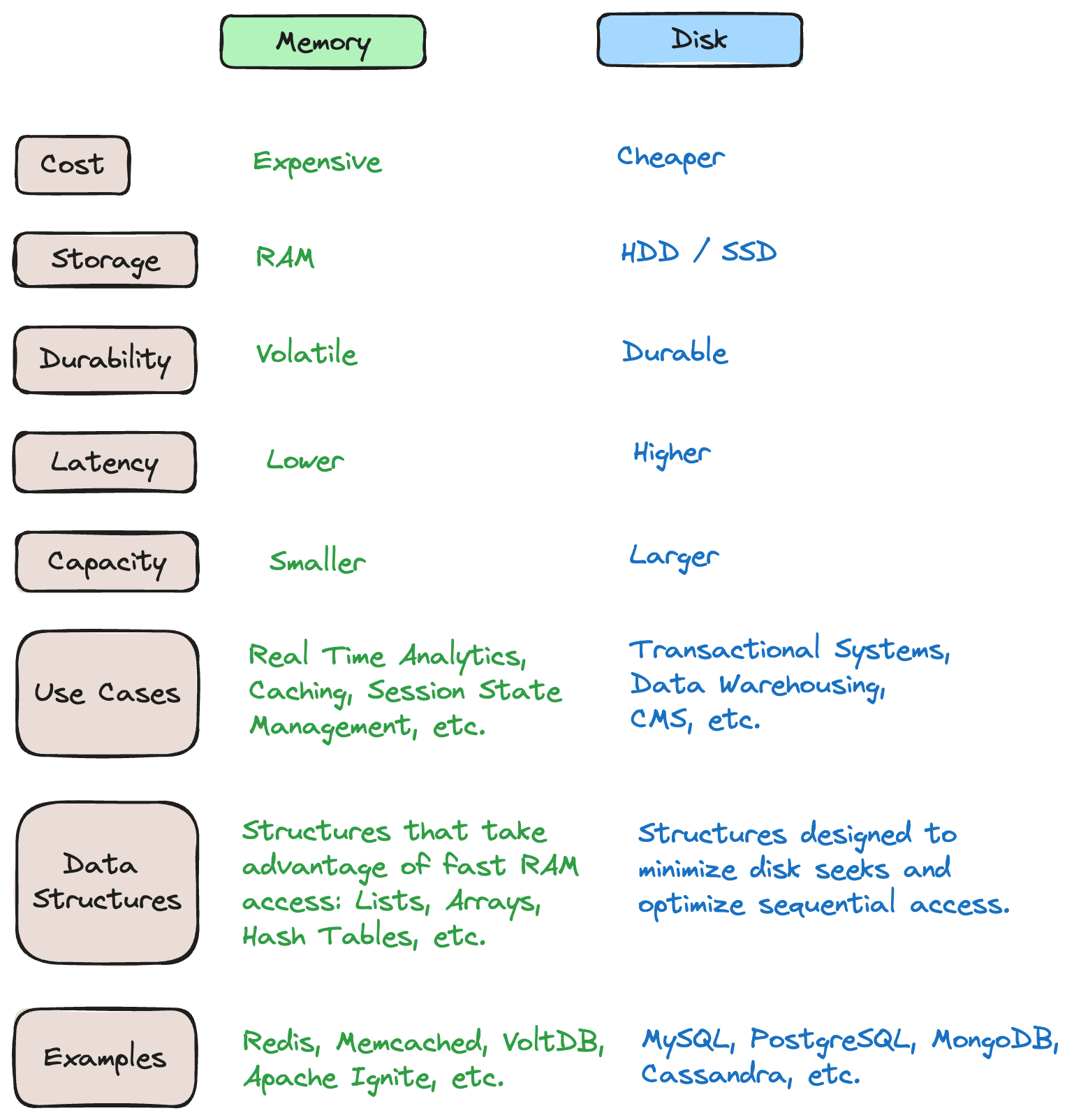
* Note that most in-memory databases do offer some durability by using the disk to store logs to recover and prevent permanent loss of volatile data.
The focus of this post will be on the Data Structures used to design such databases. While the In-Memory data structures are familiar and easier to implement, designing the data structures for Disk-Based DBMS is more involved with the goal of providing efficient access speeds along with the persistent durability.
How Disk is Organized Overview
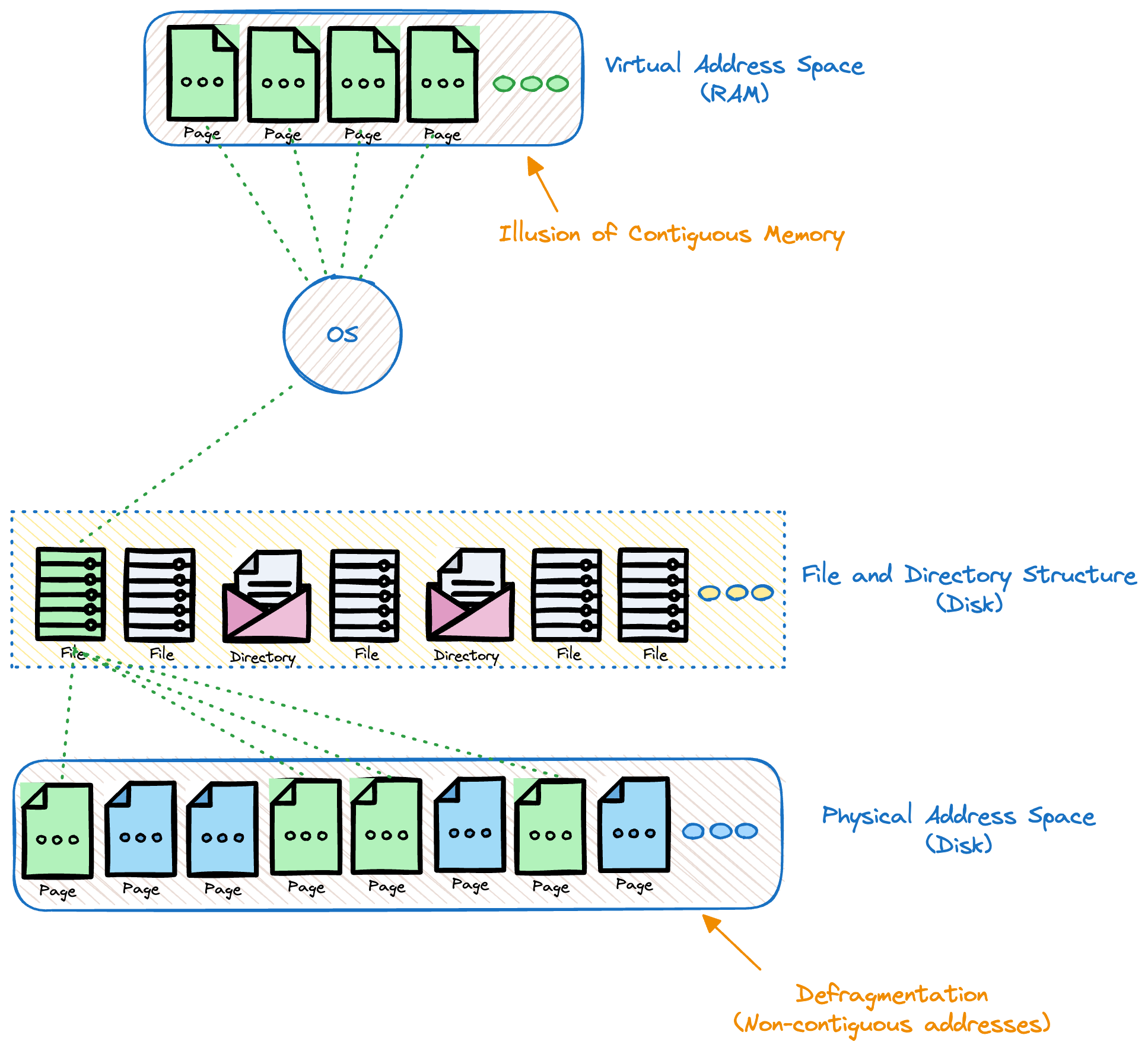
The following is a high level overview of how data is read from disk:
Data stored as files.
Files are read to memory and written to disk in terms of Pages/Blocks.
The page size is a fundamental unit of data transfer between disk and memory.
The operating system defines a fixed-size unit called a "page." Common page sizes range from 4 KB to 16 KB, with 4 KB being a typical choice
Memory Buffering: The read data is often buffered in memory. This means that the operating system loads entire pages into memory, even if the application only requested a smaller portion. Subsequent reads or writes to the same page can then be satisfied from the buffered data in memory, improving performance. Similarly, the write data may be buffered to aggregate towards the page/block size to reduce the no of Disk write operations.
Page Alignment: File data on disk is often organized in page-sized blocks. When a file is read or written, it aligns with these page-sized blocks for efficiency.
Data Fragmentation (Refer below)
Data and Index Files
Database systems use files for storing the data using implementation specific formats: Data Files store data records, while index files store record metadata and use it to locate records in data files. There are different ways in which the database may organize the data:
Index Organized (Most Popular)
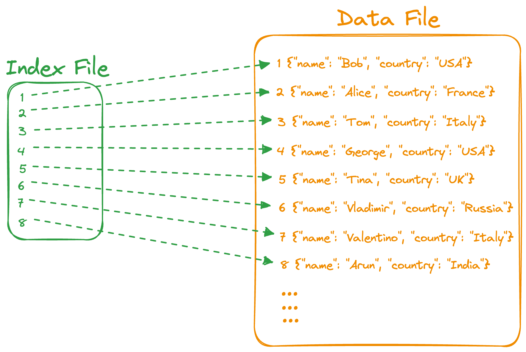
Above is a simple representation of how the data is logically stored under the Index-Organized scheme. The data is stored in Index order. This index can be an auto-generated Primary index or configured via the application developer.
Insert Query: The new record is inserted. The Index is updated to include the reference to the record location by the indexing key.
Read Query: Index is used to identify the record location.
Range Query: Since the data is stored in index order, range traversal is feasible.
Delete Query: The record is located using the index. The index is updated to remove the reference to the deleted record. DB systems may implement a further reorganization of the data files to clean up unreferenced records.
Primary vs Secondary Indexes
Primary Indexes ensure the uniqueness of each record in the table while Secondary Indexes may hold several entries per search key.
The data file is usually ordered based on the primary key (clustered index). Refer Clustered vs Non-Clustered Indexes.
There can only be one primary index and multiple secondary indexes.
Secondary Indexes can use the Primary Index as an Indirection. 2 ways in which secondary indexes reference data:
Direct data reference: Reduce the no of disk seeks, but cost of updating pointers whenever the record is updated or relocated.
Primary Index as an Indirection: reduce cost of pointer updates, higher cost on the read path.
Clustered vs Non-Clustered Indexes
A clustered index determines the physical order of data.
A non-clustered index is a separate structure from the data rows. It contains a sorted list of key values and pointers to the corresponding data.
Only one clustered index, multiple non-clustered indexes.
Clustered indexes faster for range queries, while non-clustered indexes offer faster inserts/updates/deletes because the data itself does not need to be reorganized.
Heap Organized
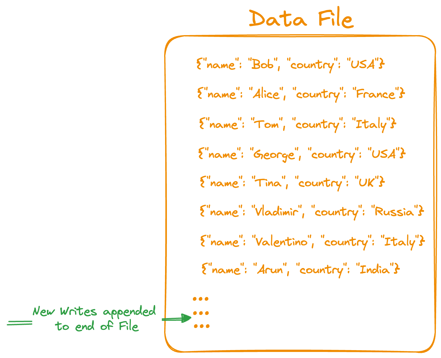
Above is a simple representation of how the data is logically stored under the Heap-Organized scheme. The data is not stored in any particular order.
Insert Query: Inserts are efficient with new records appended to the end of the data file.
Read Query: Since no order is maintained, Reads need to scan through all records to identify the requested record.
Range Query: Since no order is maintained, requires scanning all the records in the data file.
Delete Query: The record is located using a full scan. The record data is deleted. DB systems may further implement compaction to remove fragmentation of the data files due to deleted records.
Hash Organized
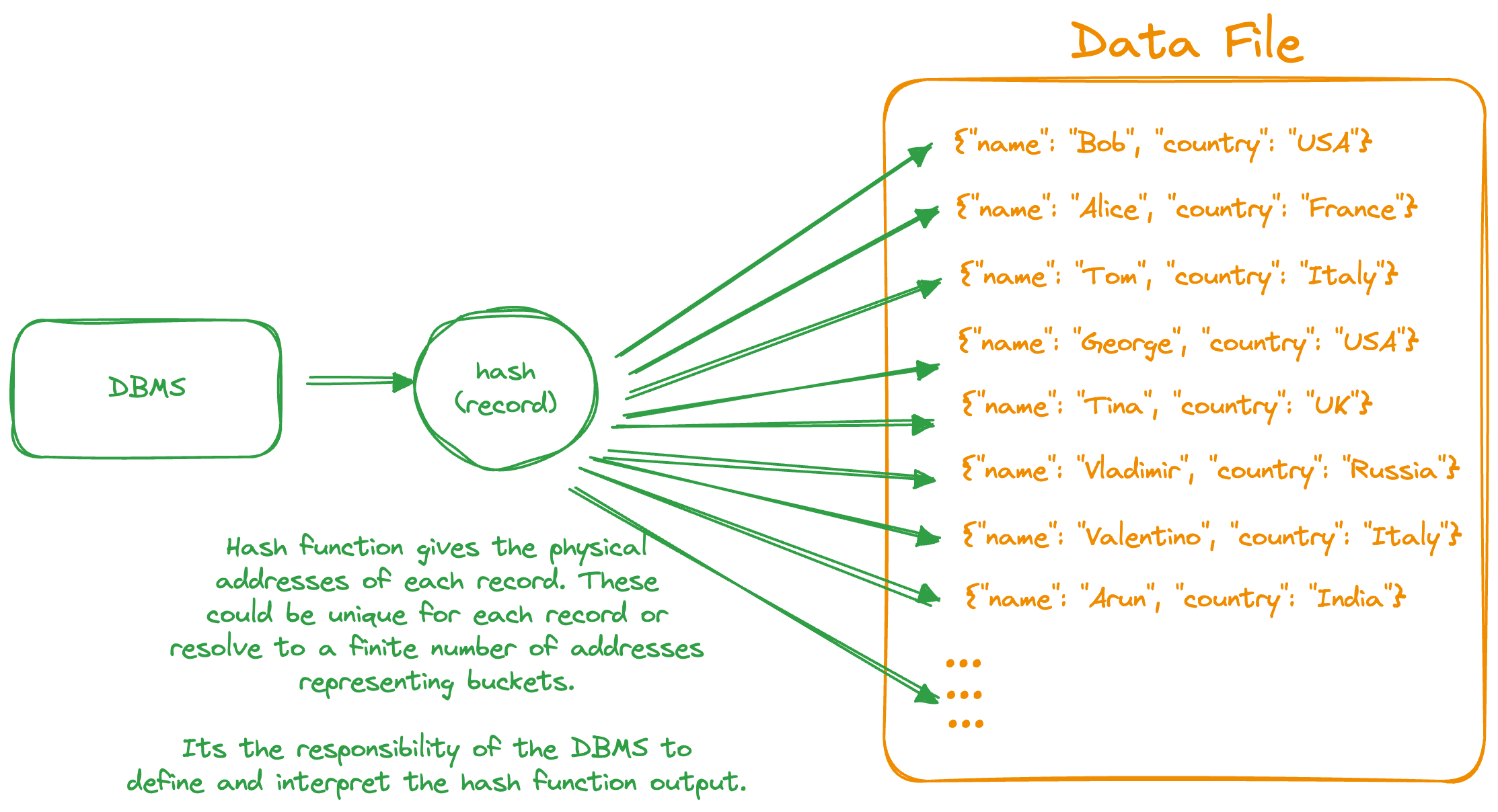
Above is a simple representation of how the data is logically stored under the Hash-Organized scheme. This scheme is efficient for exact-match search type queries.
Insert Query: Inserts are efficient with the new records written to the location provided by the hash function.
Read Query: Efficient Reads as the hash function points to the record location.
Range Query: Not suited for range queries, since hash function doesn’t preserve order, and neighbouring records may not be stored close to each other.
Delete Query: Efficient deletes as the hash function points to the record location.
Having glimpsed how the data is laid out on the disk, followed by different indexing strategies, let us review the two most widely used data structures for Disk-Based Databases.
B-Trees
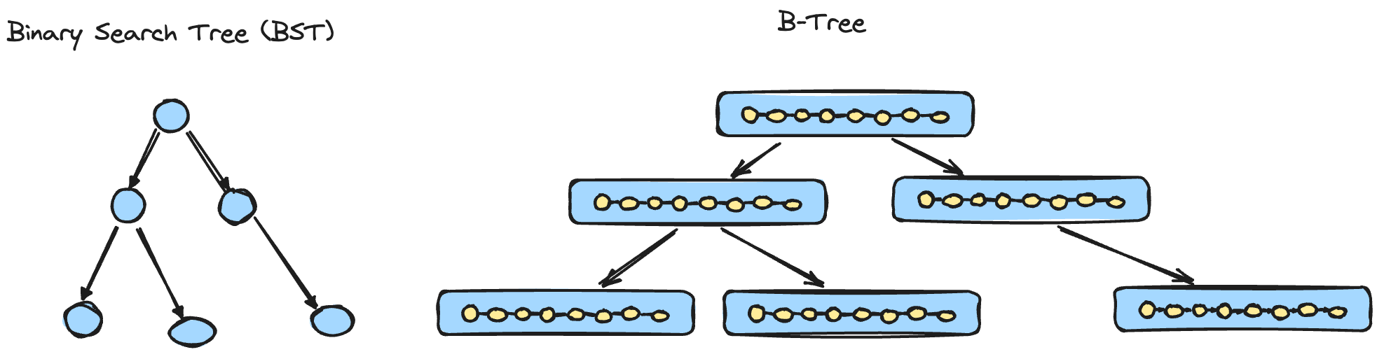
“B-Trees build upon the foundation of Balanced BSTs and are different in that they have higher fanout (have more child nodes) and smaller height.” - Database Internals by Alex Petrov
A BST node generally contains a single key, while a B-Tree contains a large number of keys (high fanout)
A BST node has two child pointers (left, right). A B-Tree node with ‘n‘ keys will have ‘n+1‘ child pointers.
Keys inside the B-Tree node are sorted to allow the application of Binary Search when looking for a key inside a B-Tree node.
B-Trees maintain balance by ensuring that all leaf nodes are at the same level.
Why B-Trees for Disk Based Storage Systems?
As we outlined under #How Disk is Organized Overview, Disk I/O operations typically read and write data in fixed-size blocks or pages.
A B-Tree is designed to store as much data as possible in a single node so that each node fits within a disk page.
When a node is accessed, the entire node (and all its keys and pointers) is loaded into memory. This reduces the number of disk reads needed since multiple keys and pointers are retrieved in a single I/O operation.
B-Trees allow efficient caching, taking advantage of locality of reference. Once a node is read into memory, it can be cached, allowing future operations on nearby keys to be faster because they might not require additional disk I/O
B-Tree Operations
A B-Tree Node with ‘k’ keys has a branching factor of ‘k+1‘ (k+1 child nodes).
Therefore the maximum no of B-Tree nodes at height ‘h‘ is kh.
Therefore the maximum no. of keys that can be stored in a B-Tree of height ‘h‘ is
(kh - 1) * k .
Most databases can fit into a B-Tree that is 3-4 levels deep, so you don’t need to follow many page references to find the page you are looking for. (A 4-level tree of 4KB pages with a branching factor of 500 can store up to 256 TB) - Designing Data-Intensive Applications by Martin Kleppmann.
Get Key
The B-Tree lookup complexity is generally denoted as logN. logkN to chase the page reference pointers and log2k for performing binary search within a page(node).
Range Scan
On each level of the B-Tree, we get a more detailed view of the tree.
The range scan begins by locating the starting key of the range, which is essentially a lookup operation (Get) in the B-Tree, which has a time complexity of logN.
Once the starting key is found, the B-Tree is traversed to collect all the keys within the specified range.
B-Trees (Read B+ Trees below) are designed for efficient sequential access, so moving from one key to the next within the same node or to an adjacent node is a relatively low-cost operation.
Updates/Deletes
The lookup algorithm defined above is used to locate the target leaf (node) and find the insertion point.
Once the target node is located, the key and value are appended to it.
Similar approach for updates/deletes.
Since B Tree nodes have a defined capacity, insertions and deletions may cause two scenarios:
Node Splits:
If inserting a new key value pair or a new page (node) pointer (Refer B+ Trees) causes an overflow, a node is split into two nodes by:
Allocating a new node
Copying half the elements from the splitting node to the new one.
Placing the new element into the corresponding node.
At the parent of the split node, add a separator key and a pointer to the new node
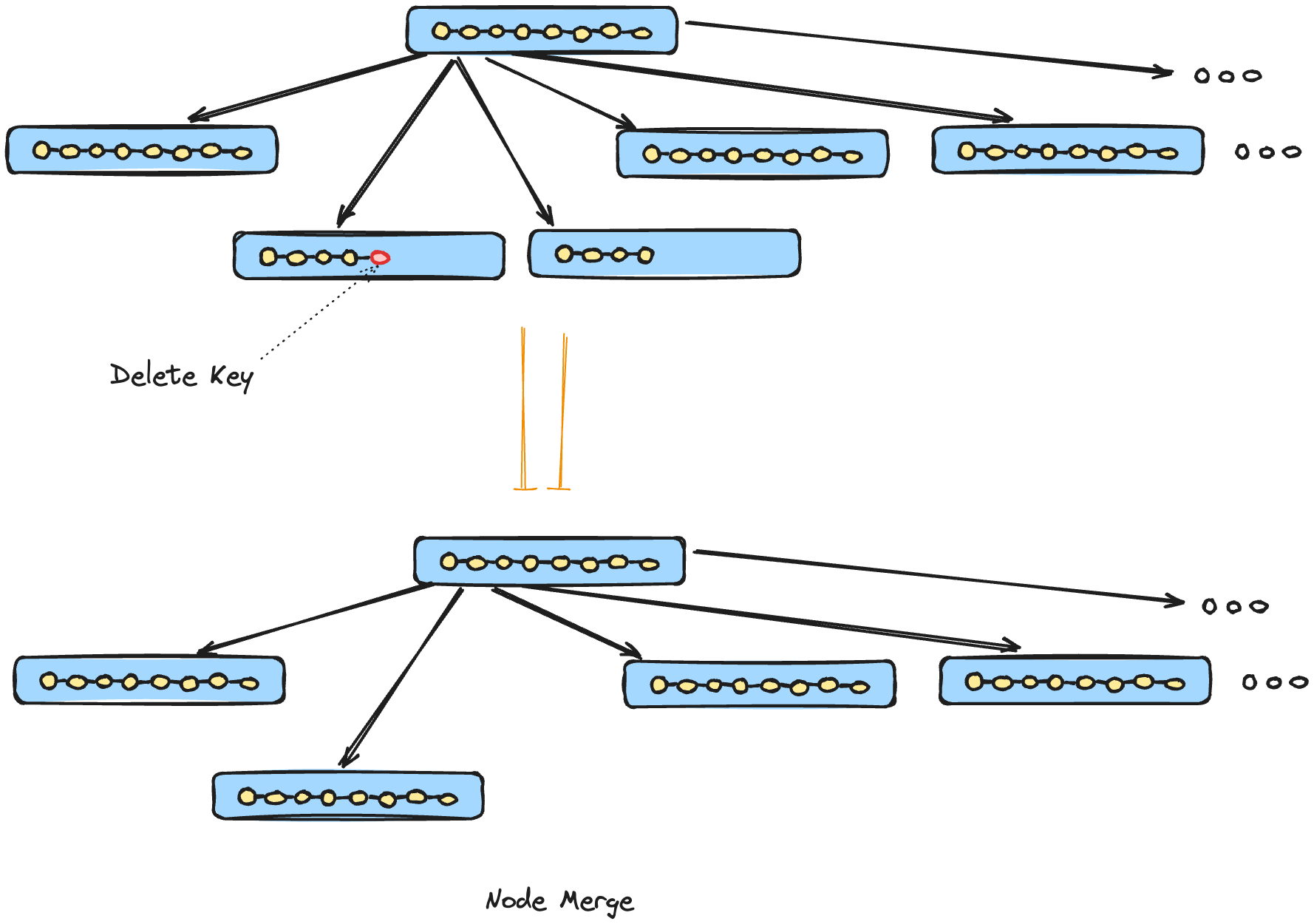
Node Merges
Deleting a key/value pair may result in two underflow scenarios:
The contents of adjacent nodes having a common parent, can fit into a single node; hence their contents should be merged.
Rebalancing: Combined contents don’t fit into a single node, and keys are redistributed between them to restore balance.
B+ Trees
B Trees allow storing values on any level: root, internal and leaf nodes.
An efficient implementation of B-Trees where values are stored only in leaf nodes is known as B+ Trees.
All operations including the retrieval of data records affect only leaf nodes and propagate to higher levels only during Node Splits and Node Merges.
Log Structured Merge Tree (LSM Tree)
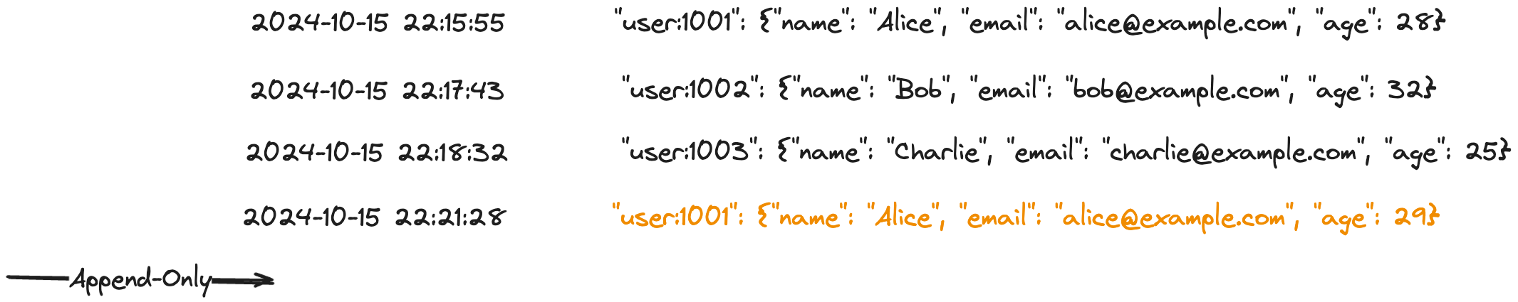
The core concept of an LSM Tree mirrors that of a log file, as both depend on 'append-only' and 'immutable' properties.
LSM Trees write immutable files and merge them together over time. These files usually contain an index of their own to help readers efficiently locate data (Refer Hash Organized Indexes).
Even though LSM Trees are often presented as an alternative to B-Trees, it is common for B-Trees to be used as the internal indexing structure for an LSM Tree’s immutable files.
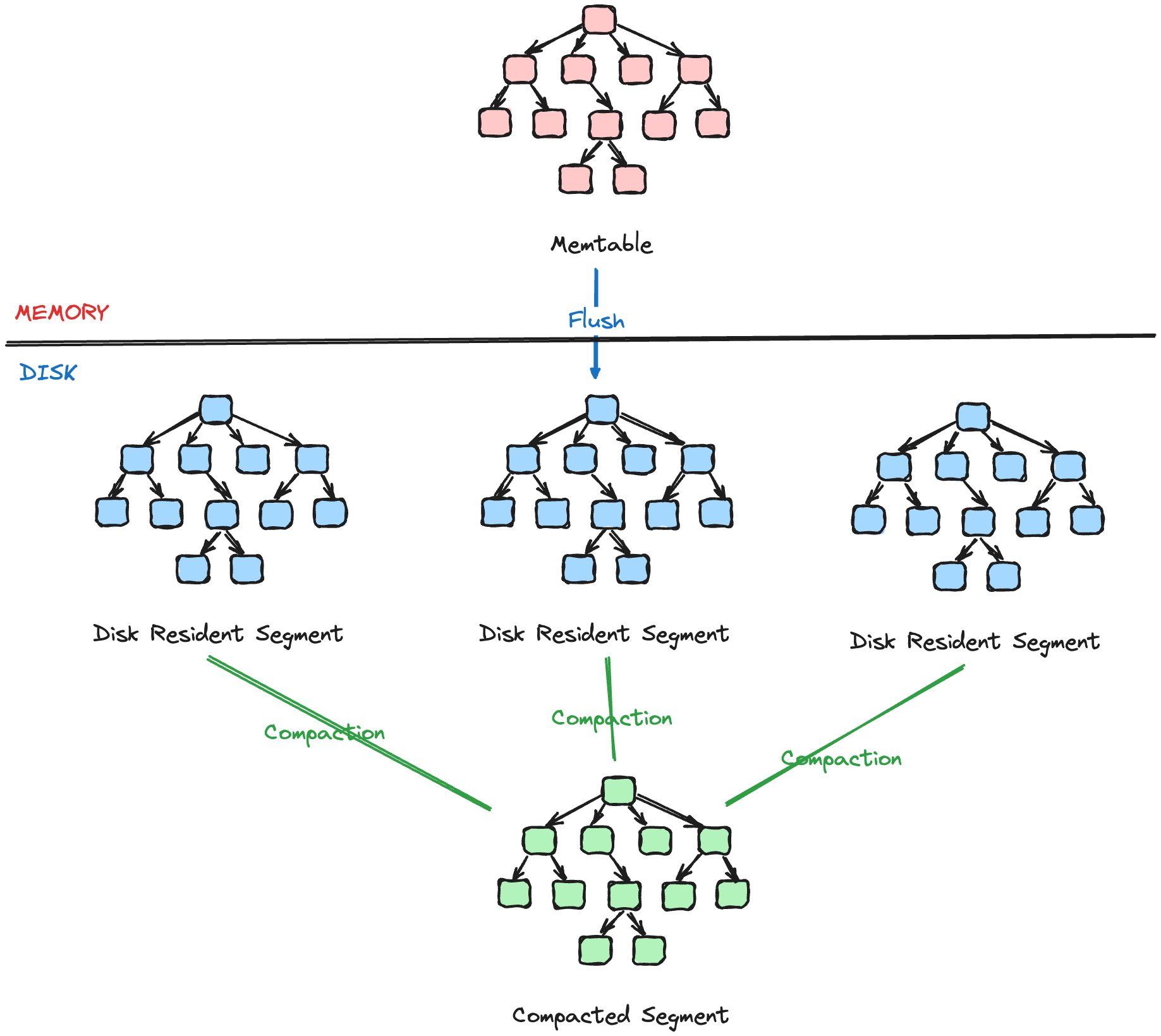
Memtable is a memory-resident, mutable component. It buffers data records and serves as a target for read and write operations. Memtable contents are persisted on disk when its size grows up to a configurable threshold. Memtable updates incur no disk access and have no associated I/O costs.
A write-ahead-log (WAL) file is used to guarantee durability of data records.
Disk-resident components are built by flushing contents buffered in memory to disk. These components are used only for reads: buffered contents are persisted, and files are never modified.
Writes against an in-memory table, Reads against disk and memory-based tables.
2-component LSM Tree: Only 1 disk component. Periodic flushes merged contents of a memory-resident segment and the disk-resident segment.
Multi-component LSM Tree: Multiple Disk components, Memtables flushed on exceeding threshold. Requires periodic merge process called Compaction.
LSM-Tree Operations
Updates/Deletes
Insert, Update and Delete operations do not require locating data records on disk. Instead, redundant records are reconciled during the read.
However, deletes need to be recorded explicitly. This is done by inserting a special delete entry sometimes called a tombstone. The reconciliation process picks up tombstones, and filters out the records. The compaction process also ignores these records when merging multiple segments.
Lookups
Generally the contents of the disk-resident segments are stored in a sorted fashion. A multiway-merge sort algorithm is used. The algorithm may use a priority queue type data structure such as a min-heap:
Fill the PQ with the first items from each iterator (per segment).
Take the smallest element (head) from the queue.
Refill the queue from the corresponding iterator (segment), unless this iterator is exhausted.
Overall lookup complexity is NlogN.
What happens during Merge conflicts?: Reconciliation
A scenario where different segments may hold data records for the same key, such as updates and deletes. The PQ implementation should be able to allow multiple values associated with the same key.
We need to understand which data value takes precedence. Data records hold metadata necessary for this, such as timestamps.
The following figure reproduced from the one in “Database Internal by Alex Petrov“ (Chapter 7) denotes the Read and Write Paths against the components of an LSM storage engine:
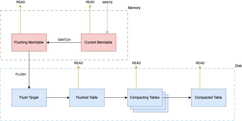
When storing data on disk in an immutable fashion (LSM), we face three problems:
Read Amplification: Resulting from a need to address multiple tables to retrieve data.
Write Amplification: Caused by continuous rewrites by the compaction process.
Space Amplification: Arising from storing multiple records associated with the same key.
One of the popular cost models for storage structures: RUM Conjecture takes these 3 factors into consideration. RUM Conjecture states that reducing two of these overheads inevitably leads to change for the worse in the third one, and that optimization can be done only at the expense of one of the three parameters.
Ordered vs Unordered LSM Storage
Sorted String Tables (SSTables)
Data records in SSTables are sorted and laid out in key order. SSTables usually consist of two components: index files and data files (Refer Data and Index Files section above).
Index files are implemented using some structure allowing logarithmic lookups, such as B-Trees, or constant-time lookups, such as hash-tables.
SSTables offer support for Range Scans.
Unordered LSM Storage
Unordered stores generally do not require a separate log and allow us to reduce the cost of writes by storing data records in insertion order.
Such stores use a hash-table like data structure (keydir), which holds references to the latest data records for the corresponding keys. Old data records may still be present on disk, but are not referenced from keydir, and are garbage collected during compaction. This approach is used in one of the storage engines (Bitcask) used in Riak. This approach does not offer support for Range Scans.
WiscKey is an interesting storage engine that attempts to preserve the write and space advantages of unordered storage, while still allowing us to perform range scans.
Conclusion: Comparing B-Trees and LSM-Trees
LSM Trees are immutable and append-only, meaning data is never modified in place; instead, new records are appended. In contrast, B-Trees perform in-place updates, modifying records directly on disk.
Storage Structure and Data Update: LSM Trees write data sequentially and use periodic merging for reconciliation. B-Trees locate and update data records at their original disk locations, resulting in more random I/O operations.
Read vs. Write Optimization: B-Trees are optimized for faster reads by locating data in place, but write performance suffers as updates require locating the record first. LSM Trees, optimized for write performance, avoid locating records by appending new data but require reconciliation across multiple versions during reads.
I/O Pattern: B-Trees primarily involve random I/O for reads and updates, rewriting entire pages even for minor changes. LSM Trees, by contrast, perform more sequential I/O and avoid page rewrites, enhancing their write performance.
Performance Comparison: Generally, LSM Trees perform better for writes and B-Trees for reads due to their design trade-offs.
Storage Efficiency: LSM Trees can achieve better compression and smaller file sizes by minimizing fragmentation with leveled compaction. B-Trees often waste space due to page splits and unutilized space, which accumulates as fragmentation over time.
Compaction Overhead: A downside to LSM Trees is the potential for compaction processes to interfere with read/write performance, especially under heavy load. B-Trees, by comparison, offer more predictable response times, though at the cost of reduced write throughput.
Disk Bandwidth Utilization: LSM Trees require the disk’s bandwidth to be split between initial writes (e.g., logging and flushing memtables) and compaction, which intensifies with data growth. This can constrain write performance in large-scale applications.
Compaction Tuning Challenges: If compaction doesn’t keep pace with incoming writes, the number of unmerged segments on disk can grow, increasing disk space usage and slowing reads. Effective compaction tuning is critical for sustaining LSM Tree performance.
Typical Use Cases: B-Trees are commonly found in relational databases and use cases with balanced, read-optimized workloads. LSM Trees are suited to high-write, large-scale sequential workloads, such as logging and NoSQL databases.
Examples of Each: Databases with B-Trees include MySQL, PostgreSQL, SQLite, and Oracle. Those using LSM Trees include Cassandra, HBase, LevelDB, and RocksDB.